Figures

 

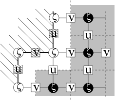
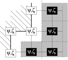
Figure 4.1: Locations of variables near a step for the SW C-grid model (left panel) and for the quasi-geostrophic (QG) model (right panel). For the SW model, dashed squares are the boundary normal velocity nodes, white disks are the vorticity nodes where the relative vorticity is specified to be zero and black disks are the vorticity nodes for which a discretized vorticity equation can be written. In grey is the region delimiting the vorticity budget domain. This region does not extend to the model boundary. Instead, there is an half cell band around the boundary (left in white) where we cannot derive any budget. A similar problem exists for the QG approximation.

 

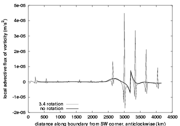
Figure 4.2: Local advective flux along the boundary ($\Cor \cdot \vdeltal/||\vdeltal||$) at 20 km resolution in a square basin for the enstrophy conserving formulation of the advection using the B combination of Table~\ref{four_cases}. The heavy-lined curve is for no rotation of the basin, the light-lined curve is for a small angle rotation of the basin ($3.4^o$) with respect to the grid. Due to the rotation angle, 4 steps occur along each side of the square and cause abrupt changes in the local advective flux.

 

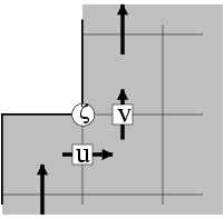
Figure 4.3: Northward flow past a forward step. The shaded area is the model domain. We consider only the two momentum nodes for which the \AM~formulation differs from the conventional formulation. The $\zeta$-point at the tip of the continent has $(i,j+1)$ indices. Arrows indicate direction of the flow.

 

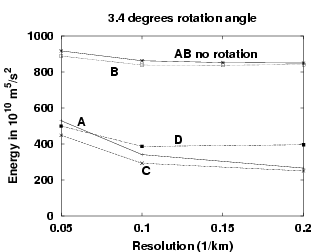
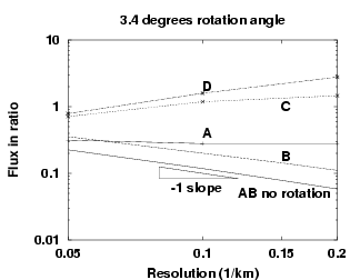
Figure 4.4: (a) Kinetic energy after spin-up and (b) ratio of $\foa$ to $\fwind$ for the four combinations combinations. Results are shown for a $3.4^o$ rotation angle of the basin. The A-B (no rotation) curve is also plotted for comparison.

 

Figure 4.5: (a) Kinetic energy after spin-up and (b) ratio of $\foa$ to $\fwind$ for the four combinations combinations. Results are shown for a $3.4^o$ rotation angle of the basin. The A-B (no rotation) curve is also plotted for comparison.

 

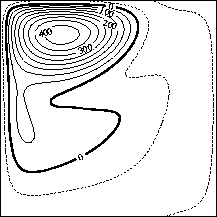
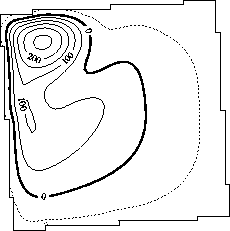
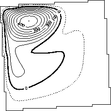
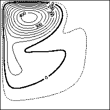
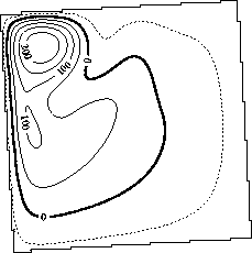
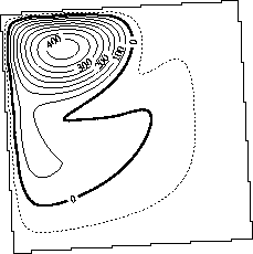
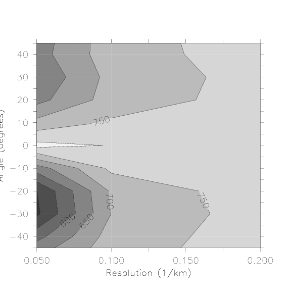
Figure 4.6: Kinetic energy after spin-up for the B combination in $10^{10}$~m$^5$/s$^2$.

 

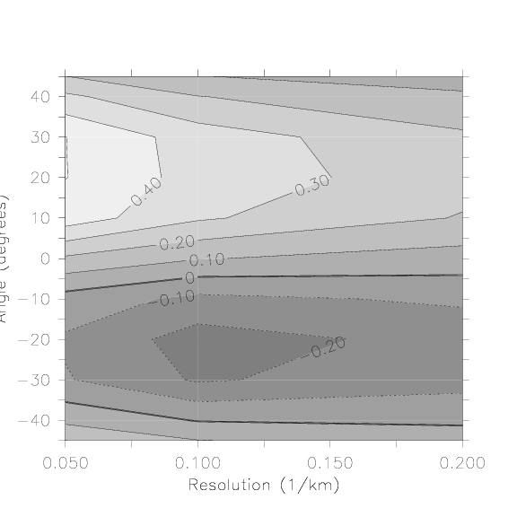
Figure 4.7: Ratio of $\foa$ to $\fwind$ for the B combination.

 

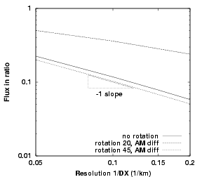
Figure 4.8: Convergence of $\foa$ with resolution for 0$^o$, 20$^o$, 45$^o$ rotation angle for the B combination.

 

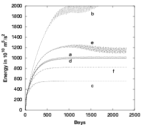
Figure 4.9: Kinetic energy during spin-up for six runs using the $J_1$ Jacobian: (a), $0^{o}$ angle at 20 km resolution; (b), $30^{o}$ angle at 20 km; (c),$-30^{o}$ angle at 20 km; (d), $0^{o}$ angle at 10 km; (e),$ 30^{o}$ angle at 10 km; (f),$-30^{o}$ angle at 10 km.

 

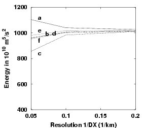
Figure 4.10: Kinetic energy after spin-up for (a) $J_3$ at $0^{o}$ rotation, (b) $J_7$ at $0^{o}$, (c) $J_3$ at $30^{o}$, (d) $J_7$ at $30^{o}$, (e) $J_3$ at $-30^{o}$, (f) $J_7$ at $-30^{o}$.

 

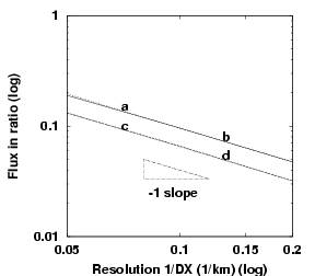
Figure 4.11: Ratio of $\foaaa$ to the wind input for (a) $J_3$ at $0^{o}$ rotation, (b) $J_7$ at $0^{o}$, (c) $J_3$ at $30^{o}$, (d) $J_7$ at $30^{o}$.

 

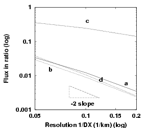
Figure 4.12: Ratio of $\fc$ to the wind input. (a-d) as described in Fig. 4.10.

 

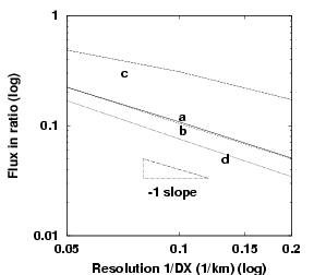
Figure 4.13: Ratio of $\foa=\foaaa + \fc$ to the wind input. (a-d) as described in Fig. 4.10.

Get the PS or PDF version here