Model Selection and Experimental Design

  

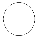
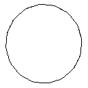
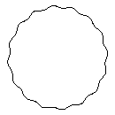
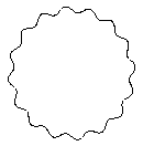
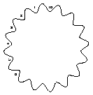
Figure 5.2: The five geometries used for our application of the SE method. The circle is deformed by super-imposition of a coastal oscillation of the form of a sine wave. For Geometry V, we label the bumps for later reference starting from the first bump west of the north-south axis passing through the center of the basin and we then proceed anticlockwise. The same labeling applies for the other geometries.

	I	II	III
IV	V

In order to test these arguments, we consider the following experiment. The set-up consists of wind-driven circulations in five different geometries (Figure 5.2). The first is a circular geometry with the radius given by L_c=500 km. The second is a perturbation of the first geometry by the addition of a wavy pattern along the coastline in the form of a sine wave. We choose the wave length to be a 1/16 of the perimeter. The amplitude of the sine wave from a crest to a trough is 12.5 km. The third geometry is the same one except that the amplitude of the sine perturbation is 25 km. The amplitude for the fourth and the fifth is respectively 50 and 100 km. The radius of curvature was computed using the simple relation:

$$\frac{\partial \mbox{\bf e}_s}{\partial s} = -\frac{1}{R_s} \mbox{\bf e}_n$$ (5.8)

where e_s and e_n are the orthonormal unit vectors associated with the directions s and n. For a sine wave given by $y=h_0 \sin (kx)$ the minimum radius of curvature is given by

$$\frac{1}{R_s}= h_0 k^2$$ (5.9)

In the context of the circular geometry, we can correct the radius by using the relation:

$$\frac{1}{R_s}= h_0 k^2 + \frac{1}{L_c}$$ (5.10)

Hence, the minimum radius of curvature for the second geometry is about 160 km and 80 km, 40 km and 20 km for the third, fourth and fifth geometries. We use three values of the eddy-viscosity ($\nu=$ 700, 300, 100 m² s^-2). The wind-forcing is the same as applied in the previous chapter for single gyre Munk problem. The Reynolds boundary number ranges therefore from 0.5 to 3.5. For comparison, Scott and Straub (1998) reached impressive values of about 35 for double gyre steady circulations with a QG model. In contrast, our maximum achieved value of R_e=3.5 is lower. However, in the context of unsteady solutions in irregular geometries using a shallow water reduced gravity model and due to our definition of V_Sv, this can be considered a high value. The inertial layer width is about 28 km whereas the viscous sublayer width varies from 40 km to 15 km. Therefore, we expect that the processes are mostly nonlinear. Since we are interested in the mean states of the circulation, when possible, we performed six year averages of the fields after a statistical steady state has been reached. This period is limited by computer resources. It is a bit short since six years represent only twice the time for a Rossby wave to cross the basin. However, we do not believe that these results would significantly differ for longer averaging period.

We first compare the results from the C-grid FD model using the promising $\delta$-$\zeta$ stress tensor formulation and the enstrophy conserving scheme (the B combination of Section 4.22) with those of the C-grid using the same advective scheme and the conventional stress tensor formulation (the A combination of Section 4.22). Figure 5.3 shows the elevation fields after a 3 year spin-up for $\nu=$ 100 m² s^-2. The circulation of the B combination is much more inertial than the circulation of the A combination. Furthermore (but not shown), the vorticity fields are very noisy in both cases. The B combination run is stopped shortly after the third year of simulation because of the depletion of the water column along the boundaries ($h<0$). Figure 5.4 shows the total energy for both combinations and the SE model. We consider the SE results to be the ``truth''. We note that the A combination is too dissipative and that the B combination is not dissipative enough. The A combination is for this geometry the combination closest to the SE results. That the B combination is not dissipative enough can be related to the fact that this particular configuration of the C-grid model specifies the vorticity to be zero at the wall and therefore, does not take into account the influence of the radius of curvature. Therefore, although the B combination was successful in the presence of steps in a rectangular geometry (where free-slip implies $\zeta=0$), this combination is no longer successful in the general case of an irregular geometry where the vorticity can be non-zero at the walls. A better way to implement the boundary condition in the FD model might be to take into account the curvature of the boundary, as we do in the SE model. This would require computing for each velocity node close to the boundary a series of coefficients associated to nearby velocity points in order to extrapolate the normal derivative of the tangential velocity along the wall (i.e., a generalization of the off-centered two point operator used in Section~\ref{app_sadourny} for enforcing free-slip along straight walls.) The C-grid however does not easily allow for such an implementation. One limitation comes from the fact that the velocity components are not discretized at the same location. This implies interpolations back and forth from the global coordinates to the local curvilinear coordinates of the components of velocity. This sort of two-way interpolation is damaging to the overall accuracy. Leakage of mass from the computational domain is also a possibility that could affect the accuracy. We therefore need a model which represents more accurately the effects of the walls. The SE model seems to be a good candidate. A second order FE model, which satisfies the LBB stability condition and which is based on the Eulerian time description, may be successful in this application as well. However, from Chapter~3, the SE model would offer a robust and faster convergence with increasing resolution at a more reasonable cost.

 

Figure 5.3: Elevation fields in the Geometry V for the C-grid model after 3 years of spin-up. On the left, the A Combination, on the right, the B combination.

 

Figure 5.3: Total energy during spin-up for the A and B combinations of the FD C-grid model and for the SE model at n_c=5 (SPOC~5) in Geometry V. $\nu=$ 100 m² s^-2.

Get the PS or PDF version here