![[*]](Images/gaucheb.gif)
![[*]](Images/droiteb.gif)
![[*]](Images/hautb.gif)
![[*]](Images/tdm.gif)
Previous: Conclusions
Next: Model vorticity budget on
Up: No Title
Table A.1:
Notations for the finite volume method
| i |
cell index |
| Voli |
cell Volume |
 |
normal oriented face length |
 |
any variable interpolated at the center of face |
| neigh |
face index for the i-cell |
|
It is possible to formulate an energy conserving scheme on a A-grid and
generalize it to a finite volume formulation (i.e., irregular domains). We
will use the notations of the latter (Table A.1).
The time integration has to be done
through an iteration process since the formulation is semi-implicit in time,
including the non-linear terms.
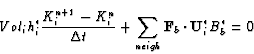
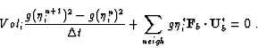
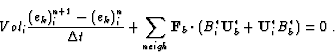
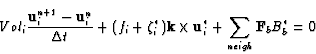 |
(7.1) |
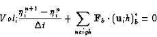 |
(7.2) |
where
 for any
  .
By multiplying A.1 by
.
By multiplying A.1 by
 ,
we get
,
we get
 |
(7.3) |
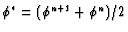
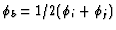
Let us define
 and use
 ,
then A.3 reads
,
then A.3 reads
 |
(7.4) |
and let us multiply A.2 by K*i and use the equivalence
 |
(7.5) |
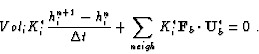
We then sum together A.4 and A.5 in order to get an equation
for the kinetic energy
 |
(7.6) |
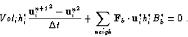
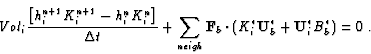
The equation for the potential energy is given by multiplying A.2 by

 |
(7.7) |
Let us define
 .
We then get the
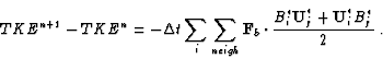
total energy equation by summing A.6 and A.7
.
We then get the
total energy equation by summing A.6 and A.7
 |
(7.8) |
Therefore, the total energy budget is
 |
(7.9) |
Hence, the conservation properties of this scheme comes from the
assumption about ,
the way we interpolate the data onto the
faces of the cells. The usual assumption is to take for any ,
 where j is the index of the neighboring cell.
Because
where j is the index of the neighboring cell.
Because
 ,
the right hand side simplifies to
,
the right hand side simplifies to
 |
(7.10) |
The right hand side vanishes for open domains. For closed domains,
some assumptions are required. If we imagine a fictitious cell on the
other side of the wall, we must have
![\begin{displaymath}\mbox{\bf F}_b \cdot
\left[ B^{*}_{i} \mbox{\bf U}^{*}_{j}
+ \mbox{\bf U}^{*}_i B^{*}_j
\right] = 0 \mbox{~.}
\end{displaymath}](Images/img493.gif) |
(7.11) |
This can be satisfied if
B*j = B*i. We are then left with satisfying
 .
This corresponds to
enforcing that the velocity is tangential at the wall.
This is a very reasonable assumption since it matches the inviscid boundary
condition. Hence, the energy can be conserved
for an A-grid scheme in absence of dissipation processes and forcing.
.
This corresponds to
enforcing that the velocity is tangential at the wall.
This is a very reasonable assumption since it matches the inviscid boundary
condition. Hence, the energy can be conserved
for an A-grid scheme in absence of dissipation processes and forcing.
In practice, this scheme only retards the upcoming of spurious modes.
In order to control the spurious modes, one idea would be to make the
scheme also conserve the enstrophy. According to
Abramopoulos abramo88, this is achievable but a unreasonable price.
Previous: Conclusions
Next: Model vorticity budget on
Up: No Title
Get the PS or PDF version here
Frederic Dupont
2001-09-11